先决条件:线性回归
本文讨论了Logistic回归的基础知识及其在Python中的实现。 Logistic回归基本上是一种监督分类算法。在分类问题中, 目标变量(或输出)y对于给定的一组特征(或输入)X只能采用离散值。
与普遍的看法相反, 逻辑回归是一种回归模型。该模型构建回归模型, 以预测给定数据条目属于编号为" 1"的类别的概率。就像线性回归假设数据遵循线性函数一样, 逻辑回归使用S型函数对数据进行建模。
仅当将决策阈值引入画面时, 逻辑回归才成为分类技术。阈值的设置是Logistic回归的一个非常重要的方面, 并且取决于分类问题本身。
阈值的决定主要受以下因素的影响:精度和召回率。理想情况下, 我们希望精度和查全率都为1, 但这很少是这种情况。如果需要进行精确召回权衡, 我们使用以下参数来决定阈值:
1.低精度/高召回率:在我们希望减少误报的数量而不必减少误报的数量的应用中, 我们选择的决策值应具有较低的Precision值或较高的Recall值。例如, 在癌症诊断应用程序中, 我们不希望任何被误诊为癌症的患者都被分类为未受影响。这是因为, 可以通过进一步的医学疾病检测到癌症的缺乏, 但是在已经被拒绝的候选人中不能检测到疾病的存在。
2.高精度/低召回率:在我们想要减少误报的数量而不必减少误报的数量的应用中, 我们选择一个具有高Precision值或低Recall值的决策值。例如, 如果我们要分类客户对个性化广告的正面还是负面反应, 则我们要绝对确定客户会对广告正面反应, 因为否则, 负面反应可能会导致潜在的销售损失。
根据类别数, Logistic回归可分为:
- 二项式:目标变量只能有2种可能的类型:" 0"或" 1", 分别表示"获胜"与"失败", "通过"与"失败", "无效"与"有效"等。
- 多项式:目标变量可以具有3种或多种不排序的可能类型(即类型没有定量意义), 例如"疾病A"与"疾病B"与"疾病C"。
- 顺序:它处理具有排序类别的目标变量。例如, 测试分数可以归类为:"非常差", "差", "好", "非常好"。在这里, 可以给每个类别一个分数, 例如0、1、2、3。
首先, 我们探讨Logistic回归的最简单形式, 即二项式Logistic回归.
二项式Logistic回归
考虑一个示例数据集, 该数据集将学习时间与考试结果对应起来。结果只能采用两个值, 即passed(1)或failed(0):
Hours(x)

     0.50

     0.75

     1.00

     1.25

     1.50

     1.75

     2.00

     2.25

     2.50

     2.75

     3.00

     3.25

     3.50

     3.75

     4.00

     4.25

     4.50

     4.75

     5.00

     5.50


     Pass(y)

     0

     0

     0

     0

     0

     0

     1

     0

     1

     0

     1

     0

     1

     0

     1

     1

     1

     1

     1

     1
所以, 我们有
即y是分类目标变量, 只能采用两种可能的类型:" 0"或" 1"。
为了概括我们的模型, 我们假设:
数据集具有" p"个特征变量和" n"个观测值。
特征矩阵表示为:
这里,

表示的值

功能

观察。
在这里, 我们保持租赁的惯例

=1。(请继续阅读, 稍后你将了解逻辑)。

观察,

, 可以表示为:

代表的预期响应

观察, 即

。我们用来计算的公式

叫做
假设
.
如果你已经进行了线性回归, 你应该记得在线性回归中, 我们用于预测的假设是:
其中
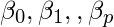
是回归系数。
让回归系数矩阵/向量

是:
然后, 以更紧凑的形式
现在取1的原因非常清楚。我们需要做一个矩阵乘积, 但是在原始假设公式中并没有实际相乘的结果。因此, 我们定义= 1。
现在, 如果我们尝试对上述问题应用线性回归, 则可能会使用上面讨论的假设获得连续值。而且, 对于

取大于1或小于0的值。
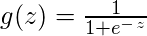
因此, 对分类假设进行了一些修改:
其中
叫做
物流功能
或者
乙状结肠功能
.
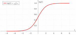
这是显示g(z)的图:
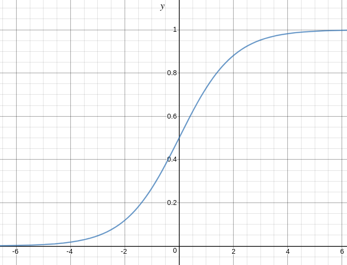
我们可以从上图推断:
g(z)趋于1

g(z)趋于0, 因为

g(z)始终在0到1之间
因此, 现在, 我们可以为2个标签(0和1)定义条件概率

观察为:
我们可以更紧凑地编写为:
现在, 我们定义另一个术语,
参数的可能性
如:
给定一个模型和特定的参数值(此处为), 似然率不过是数据的概率(训练示例)。它针对的每个可能值来衡量数据提供的支持。我们通过将所有给定值相乘来获得它。
为了简化计算, 我们采用
对数似然
:
成本函数
对数回归与参数似然性成反比。因此, 我们可以使用对数似然方程来获得成本函数J的表达式:
我们的目的是估计

从而使成本函数最小化!
使用梯度下降算法
首先, 我们取

每一个

导出随机梯度下降规则(此处仅显示最终的导出值):
在此, y和h(x)分别表示响应向量和预测响应向量。也,

是代表观测值的向量

特征。
现在, 为了得到最小

,
其中

叫做
学习率
并且需要明确设置。
让我们在样本数据集上查看上述技术的python实现(从以下位置下载)
这里
):
2.25 2.50 2.75 3.00 3.25 3.50 3.75 4.00 4.25 4.50 4.75 5.00 5.50
import csv
import numpy as np
import matplotlib.pyplot as plt


def loadCSV(filename):
     '''
     function to load dataset
     '''
     with open (filename, "r" ) as csvfile:
         lines = csv.reader(csvfile)
         dataset = list (lines)
         for i in range ( len (dataset)):
             dataset[i] = [ float (x) for x in dataset[i]]
     return np.array(dataset)


def normalize(X):
     '''
     function to normalize feature matrix, X
     '''
     mins = np. min (X, axis = 0 )
     maxs = np. max (X, axis = 0 )
     rng = maxs - mins
     norm_X = 1 - ((maxs - X) /rng)
     return norm_X


def logistic_func(beta, X):
     '''
     logistic(sigmoid) function
     '''
     return 1.0 /( 1 + np.exp( - np.dot(X, beta.T)))


def log_gradient(beta, X, y):
     '''
     logistic gradient function
     '''
     first_calc = logistic_func(beta, X) - y.reshape(X.shape[ 0 ], - 1 )
     final_calc = np.dot(first_calc.T, X)
     return final_calc


def cost_func(beta, X, y):
     '''
     cost function, J
     '''
     log_func_v = logistic_func(beta, X)
     y = np.squeeze(y)
     step1 = y * np.log(log_func_v)
     step2 = ( 1 - y) * np.log( 1 - log_func_v)
     final = - step1 - step2
     return np.mean(final)


def grad_desc(X, y, beta, lr = . 01 , converge_change = . 001 ):
     '''
     gradient descent function
     '''
     cost = cost_func(beta, X, y)
     change_cost = 1
     num_iter = 1

     while (change_cost> converge_change):
         old_cost = cost
         beta = beta - (lr * log_gradient(beta, X, y))
         cost = cost_func(beta, X, y)
         change_cost = old_cost - cost
         num_iter + = 1

     return beta, num_iter


def pred_values(beta, X):
     '''
     function to predict labels
     '''
     pred_prob = logistic_func(beta, X)
     pred_value = np.where(pred_prob> = . 5 , 1 , 0 )
     return np.squeeze(pred_value)


def plot_reg(X, y, beta):
     '''
     function to plot decision boundary
     '''
     # labelled observations
     x_0 = X[np.where(y = = 0.0 )]
     x_1 = X[np.where(y = = 1.0 )]

     # plotting points with diff color for diff label
     plt.scatter([x_0[:, 1 ]], [x_0[:, 2 ]], c = 'b' , label = 'y = 0' )
     plt.scatter([x_1[:, 1 ]], [x_1[:, 2 ]], c = 'r' , label = 'y = 1' )

     # plotting decision boundary
     x1 = np.arange( 0 , 1 , 0.1 )
     x2 = - (beta[ 0 , 0 ] + beta[ 0 , 1 ] * x1) /beta[ 0 , 2 ]
     plt.plot(x1, x2, c = 'k' , label = 'reg line' )

     plt.xlabel( 'x1' )
     plt.ylabel( 'x2' )
     plt.legend()
     plt.show()


if __name__ = = "__main__" :
     # load the dataset
     dataset = loadCSV( 'dataset1.csv' )

     # normalizing feature matrix
     X = normalize(dataset[:, : - 1 ])

     # stacking columns wth all ones in feature matrix
     X = np.hstack((np.matrix(np.ones(X.shape[ 0 ])).T, X))

     # response vector
     y = dataset[:, - 1 ]

     # initial beta values
     beta = np.matrix(np.zeros(X.shape[ 1 ]))

     # beta values after running gradient descent
     beta, num_iter = grad_desc(X, y, beta)

     # estimated beta values and number of iterations
     print ( "Estimated regression coefficients:" , beta)
     print ( "No. of iterations:" , num_iter)

     # predicted labels
     y_pred = pred_values(beta, X)

     # number of correctly predicted labels
     print ( "Correctly predicted labels:" , np. sum (y = = y_pred))

     # plotting regression line
     plot_reg(X, y, beta)
Estimated regression coefficients: [[ 1.70474504 15.04062212 -20.47216021]]
No. of iterations: 2612
Correctly predicted labels: 100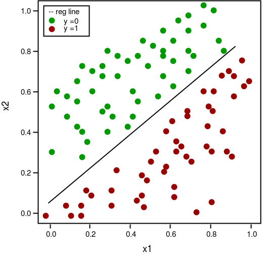
注意:梯度下降是多种估算方法之一

.
基本上, 这些是更高级的算法, 一旦你定义了成本函数和梯度, 就可以轻松地在Python中运行。这些算法是:
- BFGS(Broyden–Fletcher–Goldfarb–Shanno算法)
- L-BFGS(类似于BFGS, 但使用的内存有限)
- 共轭梯度
与梯度下降相比, 使用这些算法中的任何一种的优点/缺点:
- 优点
- 不需要选择学习率
- 通常运行得更快(并非总是如此)
- 可以从数字上为你近似渐变(不一定总是很好)
- 缺点
- 更复杂
- 除非你了解细节, 否则更多是黑匣子
多项式Logistic回归
在多项式Logistic回归中, 输出变量可以具有
超过两个可能的离散输出
。考虑一下
数字数据集
。在此, 输出变量是数字值, 可以取不到(0、12、3、4、5、6、7、8、9)中的值。
下面给出了使用scikit-learn对数字数据集进行预测的多项式Logisitc回归的实现。
from sklearn import datasets, linear_model, metrics

# load the digit dataset
digits = datasets.load_digits()

# defining feature matrix(X) and response vector(y)
X = digits.data
y = digits.target

# splitting X and y into training and testing sets
from sklearn.model_selection import train_test_split
X_train, X_test, y_train, y_test = train_test_split(X, y, test_size = 0.4 , random_state = 1 )

# create logistic regression object
reg = linear_model.LogisticRegression()

# train the model using the training sets
reg.fit(X_train, y_train)

# making predictions on the testing set
y_pred = reg.predict(X_test)

# comparing actual response values (y_test) with predicted response values (y_pred)
print ( "Logistic Regression model accuracy(in %):" , metrics.accuracy_score(y_test, y_pred) * 100 )
Logistic Regression model accuracy(in %): 95.6884561892最后, 需要考虑以下有关Logistic回归的要点:
- 不假设因变量和自变量之间存在线性关系, 但确实假设解释变量的对数和响应.
- 自变量甚至可以是原始自变量的幂项或其他一些非线性变换。
- 因变量不需要是正态分布的, 但通常假定它是来自指数族的分布(例如, 二项式, 泊松, 多项式, 正态等);二元逻辑回归假设响应的二项式分布。
- 不需要满足方差的均匀性。
- 错误必须是独立的, 但不能正态分布。
- 它使用最大似然估计(MLE)而不是普通最小二乘法(OLS)来估计参数, 因此依赖于大样本近似.
参考文献:
- http://cs229.stanford.edu/notes/cs229-notes1.pdf
- http://lsbin.com/logistic-regression-for-machine-learning/
- https://onlinecourses.science.psu.edu/stat504/node/164
如果发现任何不正确的地方, 或者想分享有关上述主题的更多信息, 请写评论。
注意怪胎!巩固你的基础Python编程基础课程和学习基础知识。
首先, 你的面试准备可通过以下方式增强你的数据结构概念:Python DS课程。